Linear L2-norm Inversion
In this chapter we put the principles of Tikhonov inversion into practice and address the numerical under-pinnings for solving the linear problem using L2 norms for the misfit and model regularization. The function to be minimized is a quadratic and a solution the inverse problem can be achieved in a single step by solving a linear system of equations. We use our flowchart to keep us on-track as we step through the basic elements. For each element we provide background that will be of use when attacking any inverse problem. These include issues about the noise and misfit, the model norm, how to solve the system numerically, how to choose a tradeoff parameter, and some basic principles for evaluating the results of the inversion and potentially carrying out an inversion with revised parameters.
1Key Points
1.1Workflow for Inversion
A successful inversion of any data set requires a workflow in which each element can be critically addressed. The quality of a final result depends upon how well each of these is implemented and in the following we elaborate on each component.
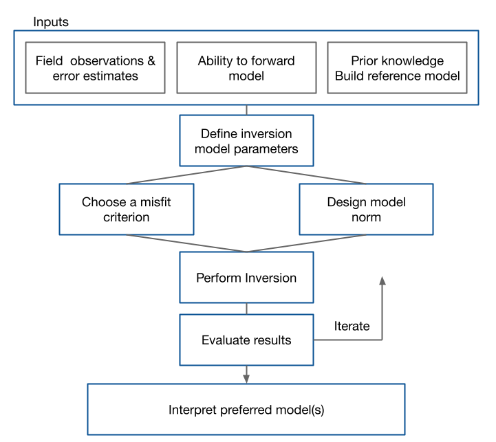
Figure 2.1: The inverse workflow displays the necessary inputs and steps taken within the generic inverse problem.
1.2Inputs
There are three boxes under the “Inputs” heading.
1.2.1Field Observations and error estimates.
This includes the obvious components such as knowing your survey acquisition parameters, the fields that are measured, and estimates of the uncertainties in the data. For instance, in a DC resistivity survey we need to know the locations of the current and potential electrodes, the transmitter current, how the electric potentials at the receiver electrodes are converted from the repetitions of the bi-polar transmitter current and stacked and subsequently processed to give a datum that corresponds to an ideal step-on transmitter current. Field logs are often required to reveal where challenges were encountered; for example electrodes could not be placed in their proposed locations because of trees, gullies, asphalt roads etc. These will later have to be modelled within the inversion, or included as “noise” in uncertainty estimates. Lastly, it is essential that all details about the subsequent processing of the data are known and importantly the final units of the data. Determining final units of the data and normalizations is traditionally one of the major hurdles for getting started on an inversion.
1.2.2Prior Knowledge
Assembling your a priori knowledge about the project area is crucial. This includes what is known about the geologic structure, lithologies, rock types and their physical property values, borehole constraints, and information for other geophysical surveys. The culmination of this work is the development of a “reference model”. Ideally this is a 3D geologic model with each unit having an estimated range of the sought physical property. Even a simple geologic sketch or a deposit model for a mineral can be valuable at this stage. For some problems the reference model might be detailed and complicated while for other problems, where little is known, the reference model might be uniform and represented by a single number. Irrespective, development of a reference model in these early stages has three important benefits:
- it will be used in the model norm to ameliorate the non-uniqueness
- when linked with the survey and forward modelling, it provides a set of predicted data that can be used as a first order check about normalizations of the data
- compiling a priori information into a reference model often clarifies what is known, and what is unknown, about the earth model. This in turn helps generate objectives for carrying out the inversion. That is, what question about the earth do we want answered when the geophysical data are included in the inversion. This becomes important in a later box in the flowchart where the parameters for inversion are specified.
1.2.3Forward modelling
The crucial component for solving an inverse problem is the ability to carry out a forward modelling to simulate data from an input model. That is, we want to evaluate
Equation 1.4 Forward mapping operation applied to an element of the model space to calculate the corresponding element in the data space .
The forward modelling needs to be accurate, which in practice means that numerical errors are less than the “noise” in the data. It must also be efficient since the forward modelling must be done many times during the course of the inversion.
To numerically simulate data we generally discretize the problem onto a mesh (1D, 2D, 3D). The cells must be sufficiently small and extend to large enough distances so that relevant boundary conditions are satisfied and that the forward modelling operator produces sufficiently accurate results. In the case of our 1D problem, you can experiment with the accuracy of the simulation by comparing data generated with a very large number of cells with data produced by discretizing with fewer cells. The inaccuracies in this case also arise because of the way the integration of the kernels is carried out for each cell; here, a mid-point rule is chosen. This becomes less accurate as the size of the cells increases and/or the frequency of the kernel function increases.
1.3Define Inversion parameters
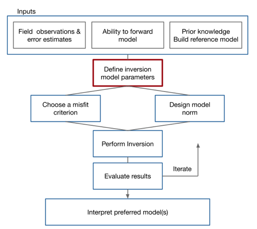
Figure 4.1: The inverse workflow (Figure 2.1), with focus on the definition of the inverse model parameters.
1.4

The mesh used for forward simulation is designed so that simulated results are high quality. We could use the same mesh for the inverse problem, as done in the notebook, but that is not necessary. Our inversion mesh could be composed of fewer cells, either by fixing the values of some cells and not including them in the inversion, or by homogenizing groups of cells. Moreover, the model parameters used for inversion might be different from those used in the forward simulation. As an example, in an electromagnetic problem the basic equations and forward simulation uses the electrical conductivity σ so . But electrical conductivity is positive and varies over orders of magnitude. Both of these attributes can be handled readily by having the inversion parameters be .
1.5Misfit criterion
As discussed in the Tikhonov section we need some way to evaluate how close the predicted data are to the observations and then a criterion for choosing a target value for that misfit.
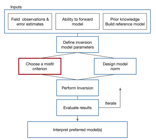
Our observed datum is defined such that where is our mathematical representation of the forward operator and is the additive noise. We want to find a model that gave rise to the data . The noise is a challenging element to quantify. It is built up from modelling errors and well as traditional experimental noise that is associated with any survey.
We first address modelling errors. The forward modelling for our physical system is as where is a function and includes the complete physics of our problem. Our numerical forward operator does not represent that exactly. Thus , where are the discrepancies between the forward operator and our mathematical representation . These discrepancies are due to a variety of factors and assumptions such as the wrong dimension (1-D, 3-D), incomplete physics, or discretization errors. The statistics of these discrepancies are problem dependent and not easily quantified.
In addition to modelling errors there are also additional additive noise \ that arises from the survey. Rewriting our observed datum with the numerical forward operator, . We can combine the additive noise in the observed data and the discrepancies in the forward operator into one statistical variable that accounts for all the noise in the system . Our observed datum is now . Clearly the statistics of is challenging to quantify but for our present purposes, we assume that each is characterized by Gaussian distribution with a zero mean and a standard deviation , that is . This is a huge simplification but we can take some comfort in the Central Limit Theorem (ref).
Consider a random variable . By taking a sum of squares we then define a new random variable, , which follows a chi-squared distribution with N-degrees of freedom. For this distribution the expected value is , the variance is , and the standard deviation is . In the next section we shall use as a misfit function for our inverse problem and its expected value as a target value.
1.6Misfit Function
There are two important components for any misfit function: specifying the metric used and determining the target misfit value. Here we will use an L2-norm, also known as the least-squares statistic, to define the data misfit function as
.
We define the data weighting matrix
and rewrite the data misfit function as
.
In reality we do not know the uncertainties within the system so we estimate them as a percentage of the observed data, plus a constant noise floor,
.
Because the data misfit function is now a variable, the expected value is approximately the number of data, . In practise we often specify our target misfit where χ is a scaler. Running inversions with allows the Tikhonov curve to be explored and helps with the decision about how well we want to fit field data where the uncertainties are only guessed at.
Assigning uncertainties to data is a critical step in a practical inversion. This point cannot be over-emphasized. Unfortunately, there is no easy one-size-fits-all recipe. Each survey is different and much care and attention needs to paid for estimating each . We offer some comments, although simplistic and general, might be useful.
- Try to balance the relative errors between data. If one datum is twice as noisy as another, this should be reflected in the relative value of assigned ε. Balancing is especially important when working with a least squares misfit. If the uncertainty for one datum is a factor η too small then its contribution to is a factor of larger than it should be and this will over-weight the effects of that datum. This is a strong motivation to use a more robust statistical measure of misfit, such as an norm but we postpone that analysis until later.
- If the relative errors in the data set are balanced then a global scaling of the uncertainties can be handled by making use of the χ factor in . The effects of reducing all of the assigned uncertainties by a factor of two is the same as working with the existing problem and setting . This is convenient we shall make frequent use of this.
- The balancing of uncertainties mentioned above holds when thinking about two data or two sets of data. Suppose you have generated a procedure where you assign
: Below we outline some The suggestion of and uncertainty is a good starting point.
1.7Model Objective Function
The model objective function can consist of one or a combination of the following model norms, discussed previously in LINK TO Linear Tikhonov Inversion:
- Smallest Model Norm
- Smallest Model Norm with Reference Model
- Smoothest Model Norm
- Smallest & Smoothest Model Norm
1.8Perform Inversion
We combine the data misfit and model objective functions into the objective function .
To solve the quadratic objective function for a single variable we calculate the derivative of the objective function with respect to the model
Consider the matrix vector equation , where is full rank and , then the above can then be considered in the form .
1.9Managing Misfit with β
In the inverse problem we minimize to find a model , but what β should we use? If the standard deviations of the data are known, then the expected value of the data misfit is the number of data, , thus the desired misfit is . We must choose β so .
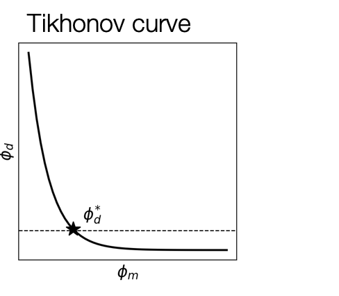

There are several options for choosing β
- Fix β - guess a constant value for β and perform the inversion
- Solve - for a logarithmic number of β, choose
- where
- Select the corner point of the L-shaped curve, point of maximum curvature
- GCV - Generalized Cross-Validation
- Cooling strategy - perform successive inversions with