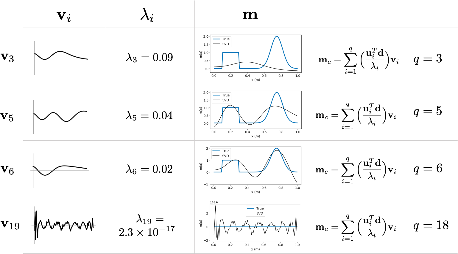
Fundamental understanding about non-uniqueness and ill-conditioning of the linear inverse problem is readily achieved with the aid of Singular Value Decomposition (SVD). In this chapter we show how this decomposition ……
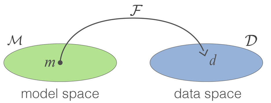
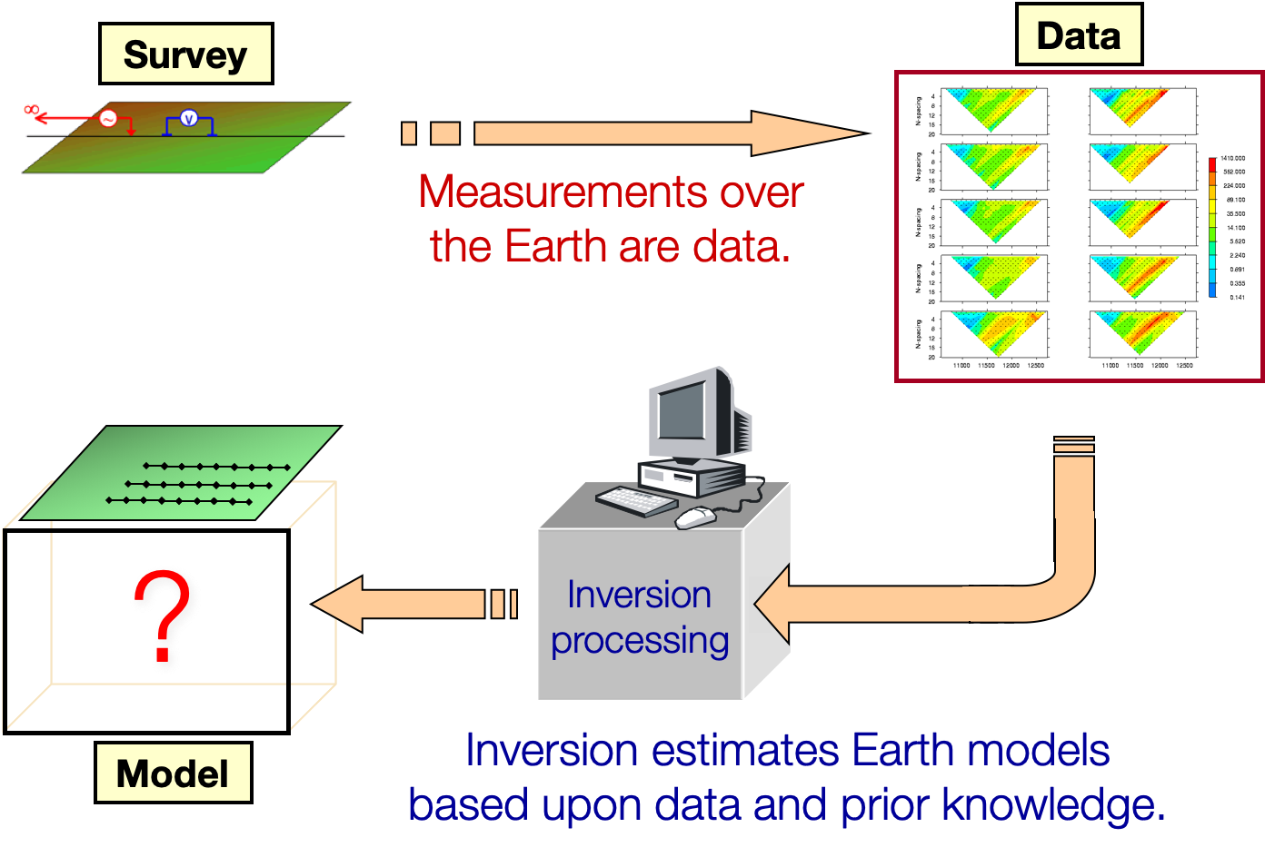
1 Recall ¶ Given observations d i o b s , i = 1 , … , N d^{obs}_i, ~i=1,\dots,N d i o b s , i = 1 , … , N ϵ j \epsilon_j ϵ j F [ m ] = d \mathcal{F}[m]=d F [ m ] = d
Find the earth model m m m
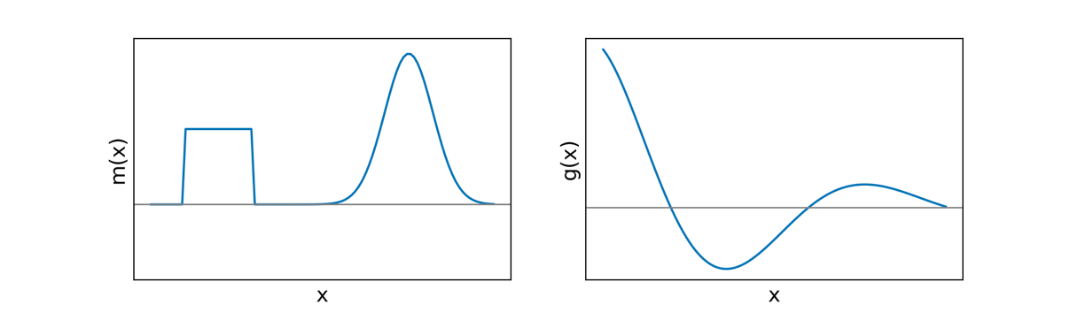
d i = ∫ v g i ( x ) m ( x ) d x g i ( x ) = e i p x c o s ( 2 π i q x ) \begin{aligned} d_i&=\int_vg_i(x)m(x)dx \\ g_i(x)&=e^{ipx}cos(2\pi iqx) \end{aligned} d i g i ( x ) = ∫ v g i ( x ) m ( x ) d x = e i p x cos ( 2 πi q x ) where d j d_j d j th datum, g j g_j g j th datum, and m m m
Each datum is an inner product of the model with the kernel function. If we evaluate one case: d i = g ⋅ m = 4.89 d_i=\mathbf{g}\cdot\mathbf{m}=4.89 d i = g ⋅ m = 4.89
1.0.3 Basic Challenges of the Inverse Problem: Non-uniqueness ¶ The data are defined such that
d i = ∑ j = 1 M G i j m j d = G m , G : ( N × M ) \begin{aligned} d_i&=\sum^M_{j=1}G_{ij}m_j \\ \mathbf{d}&=\mathbf{Gm}, ~~~G:(N\times M)\end{aligned} d i d = j = 1 ∑ M G ij m j = Gm , G : ( N × M ) Typically M > N M>N M > N
In this chapter we consider the question: How do we understand and deal with these elements?
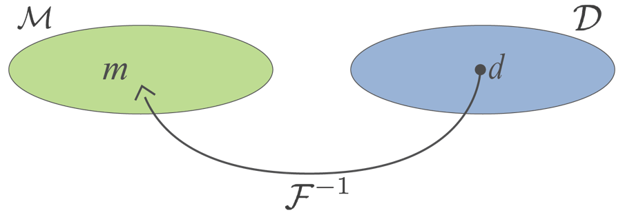
2 Solving G m = d \mathbf{Gm}=\mathbf{d} Gm = d ¶ Given G m = d \mathbf{Gm}=\mathbf{d} Gm = d G ∈ R N × M \mathbf{G}\in\R^{N\times M} G ∈ R N × M m ∈ R M \mathbf{m}\in\R^M m ∈ R M d ∈ R N \mathbf{d}\in\R^N d ∈ R N m = G − 1 d \mathbf{m}=\mathbf{G}^{-1}\mathbf{d} m = G − 1 d G \mathbf{G} G G − 1 \mathbf{G}^{-1} G − 1
For example, if we write G m = d Gm=d G m = d m 1 + 2 m 2 = 2 m_1+2m_2=2 m 1 + 2 m 2 = 2 G = [ 1 , 2 ] G=[1,2] G = [ 1 , 2 ] d = 2 d=2 d = 2 m = ( m 1 , m 2 ) T m=(m_1,m_2)^T m = ( m 1 , m 2 ) T m = G − 1 d m=G^{-1}d m = G − 1 d
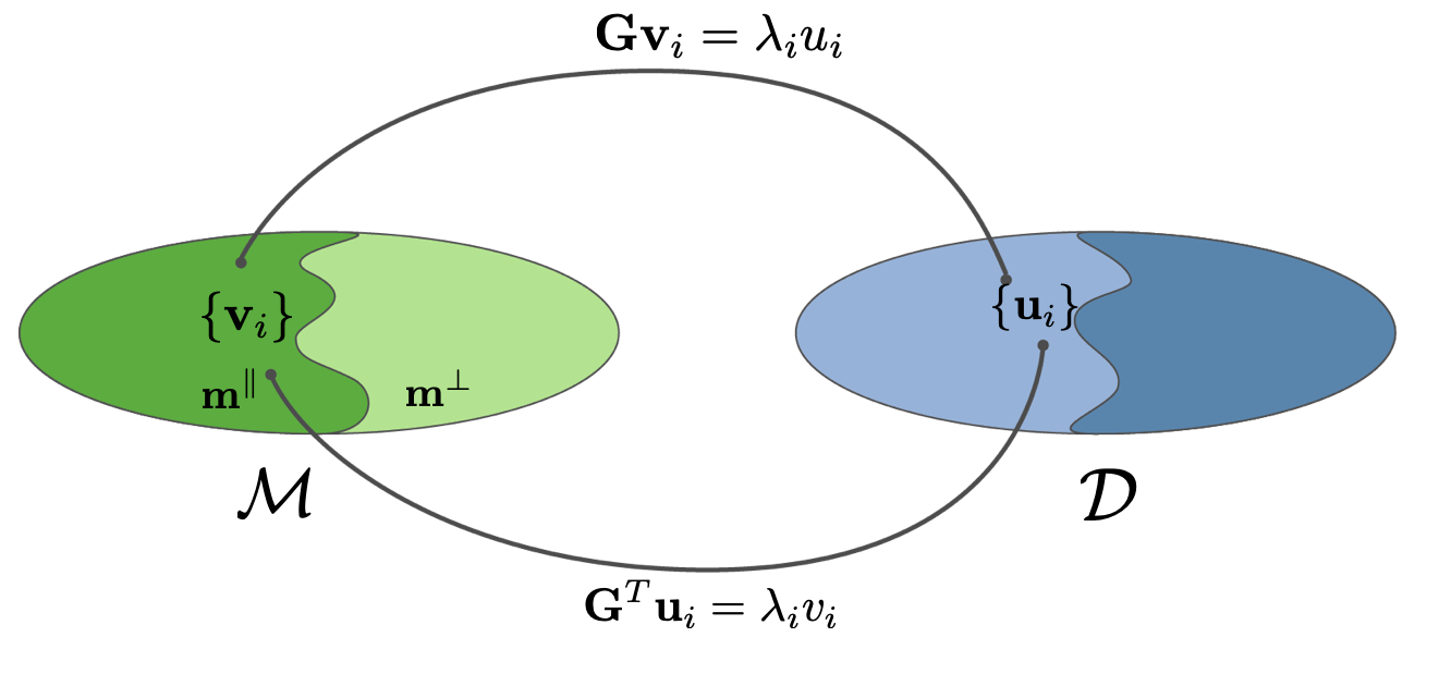
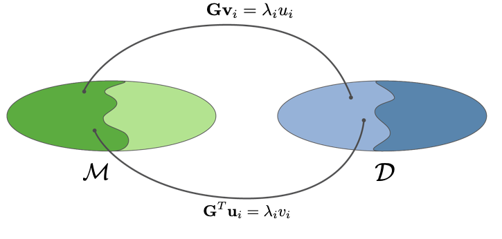
3 Singular Value Decomposition ¶ G = U p Λ V p T \mathbf{G}=\mathbf{U}_p\mathbf{\Lambda}\mathbf{V}^T_p G = U p Λ V p T
d i = ∫ v g i ( x ) m ( x ) d x d_i=\int_vg_i(x)m(x)dx d i = ∫ v g i ( x ) m ( x ) d x
G p = ( − g 1 − ⋮ − g N − ) \mathbf{G}_p =\begin{pmatrix} ~-& \mathbf{g}_1 & -~ \\ & \vdots & \\ ~-& \mathbf{g}_N & - ~\end{pmatrix} G p = ⎝ ⎛ − − g 1 ⋮ g N − − ⎠ ⎞ G \mathbf{G} G ( M × N ) (M\times N) ( M × N )
U p = ( ∣ ∣ u 1 … u p ∣ ∣ ) \mathbf{U}_p =\begin{pmatrix} |& & | \\ \mathbf{u}_1 & \dots & \mathbf{u}_p\\ |& & | \end{pmatrix} U p = ⎝ ⎛ ∣ u 1 ∣ … ∣ u p ∣ ⎠ ⎞ U p \mathbf{U}_p U p ( N × P ) (N\times P) ( N × P ) u i \mathbf{u}_i u i ( U p T U p = I p ) (\mathbf{U}_p^T\mathbf{U}_p=\mathbf{I}_p) ( U p T U p = I p )
Λ p = ( λ 1 ⋱ λ p ) \mathbf{\Lambda}_p =\begin{pmatrix} \lambda_1& & \\ & \ddots & \\ & & \lambda_p\\\end{pmatrix} Λ p = ⎝ ⎛ λ 1 ⋱ λ p ⎠ ⎞ Λ p \mathbf{\Lambda}_p Λ p ( P × P ) (P\times P) ( P × P ) λ i \lambda_i λ i ( λ 1 ≥ λ 2 ≥ … λ p > 0 ) (\lambda_1\geq\lambda_2\geq\dots\lambda_p>0) ( λ 1 ≥ λ 2 ≥ … λ p > 0 )
V p = ( ∣ ∣ v 1 … v p ∣ ∣ ) \mathbf{V}_p =\begin{pmatrix} |& & | \\ \mathbf{v}_1 & \dots & \mathbf{v}_p\\ |& & | \end{pmatrix} V p = ⎝ ⎛ ∣ v 1 ∣ … ∣ v p ∣ ⎠ ⎞ V p \mathbf{V}_p V p ( M × P ) (M\times P) ( M × P ) v i \mathbf{v}_i v i ( V p T V p = I p ) (\mathbf{V}^T_p\mathbf{V}_p=\mathbf{I}_p) ( V p T V p = I p )
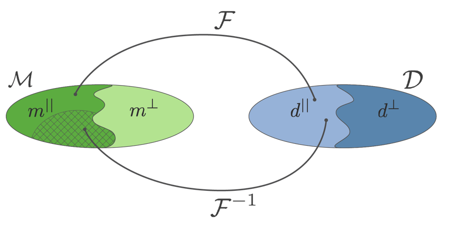
m ∥ \mathbf{m}^{\parallel} m ∥
m ⊥ \mathbf{m}^{\perp} m ⊥
3.1 Solving with SVD ¶ G m = d , G = U Λ V T U Λ V T m = d Λ V T = U T d V T m = Λ − 1 U T d V V T m = V Λ − 1 U T d \begin{aligned}\mathbf{Gm}&=\mathbf{d}, ~\mathbf{G}=\mathbf{U\Lambda V}^T \\ \mathbf{U\Lambda V}^T\mathbf{m}&=\mathbf{d}\\ \mathbf{\Lambda V}^T&=\mathbf{U}^T\mathbf{d}\\ \mathbf{V}^T\mathbf{m}&=\mathbf{\Lambda}^{-1}\mathbf{U}^T\mathbf{d}\\ \mathbf{VV}^T\mathbf{m}&=\mathbf{V}\mathbf{\Lambda}^{-1}\mathbf{U}^T\mathbf{d}\end{aligned} Gm UΛV T m ΛV T V T m VV T m = d , G = UΛV T = d = U T d = Λ − 1 U T d = V Λ − 1 U T d
Define G † = V Λ − 1 U T , m c = G † d \mathbf{G}^\dagger=\mathbf{V\Lambda}^{-1}\mathbf{U}^T, ~\mathbf{m}_c=\mathbf{G}^\dagger\mathbf{d} G † = VΛ − 1 U T , m c = G † d
m ∥ = m c = V V T m = V Λ − 1 U T d \mathbf{m}^\parallel=\mathbf{m}_c=\mathbf{VV}^T\mathbf{m}=\mathbf{V\Lambda}^{-1}\mathbf{U}^T\mathbf{d} m ∥ = m c = VV T m = VΛ − 1 U T d
m c = V Λ − 1 U T d = ∑ i = 1 N ( u i T d λ i ) v i \mathbf{m}_c=\mathbf{V\Lambda}^{-1}\mathbf{U^T}\mathbf{d}=\sum^N_{i=1}\left(\frac{\mathbf{u}_i^T\mathbf{d}}{\lambda_i}\right)\mathbf{v}_i m c = VΛ − 1 U T d = ∑ i = 1 N ( λ i u i T d ) v i
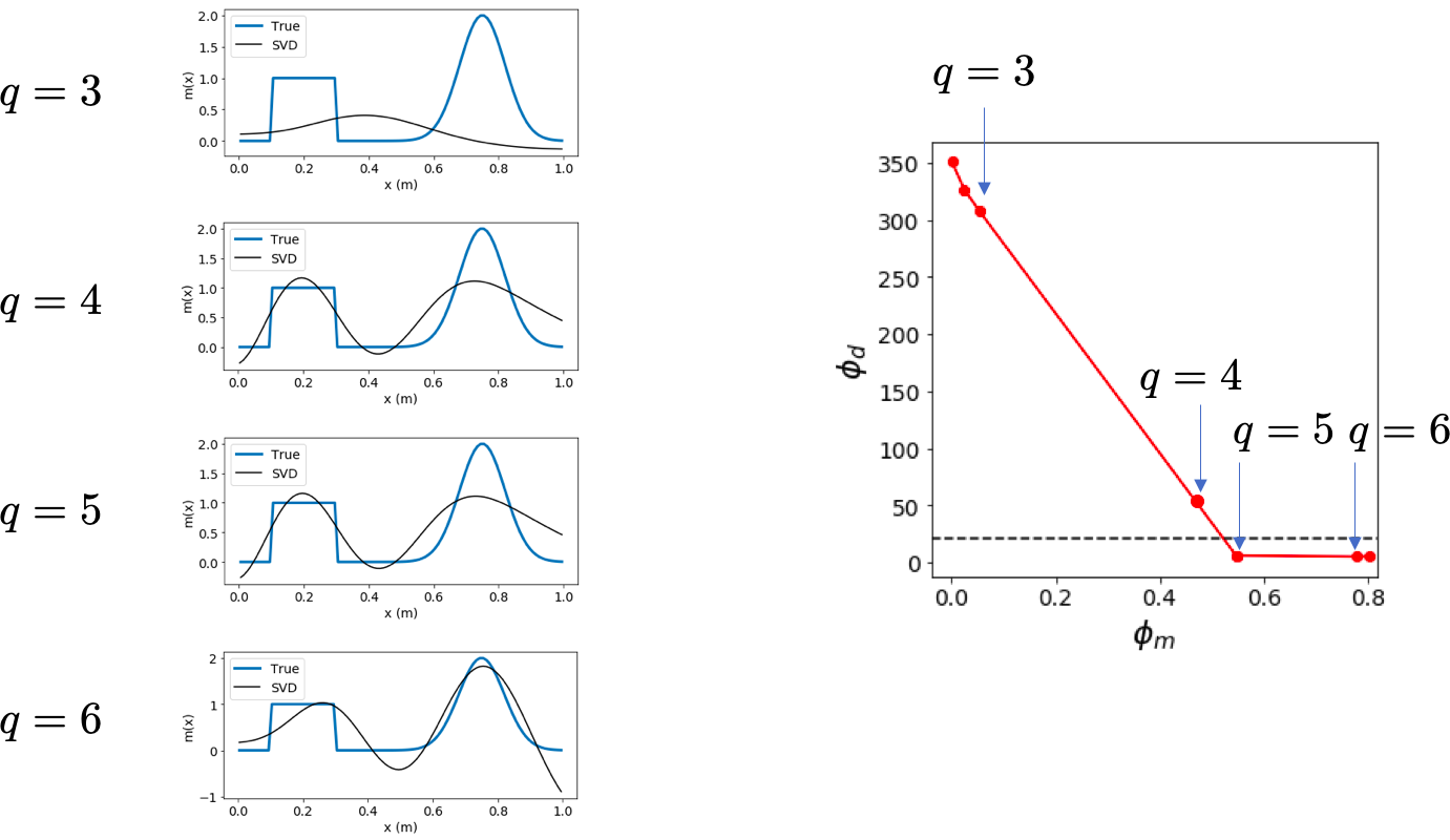
Effects: successively add vectors
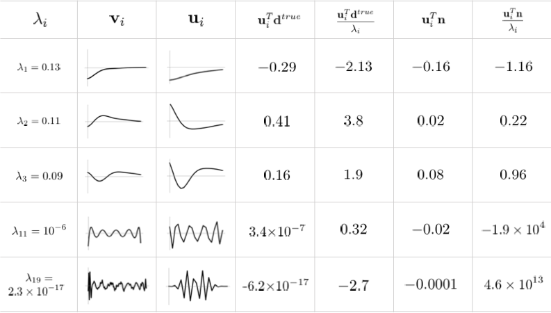
Each vector v i \mathbf{v}_i v i u i T d λ i → ∞ \frac{\mathbf{u}_i^T\mathbf{d}}{\lambda_i}\rightarrow\infty λ i u i T d → ∞ λ i → 0 \lambda_i\rightarrow0 λ i → 0
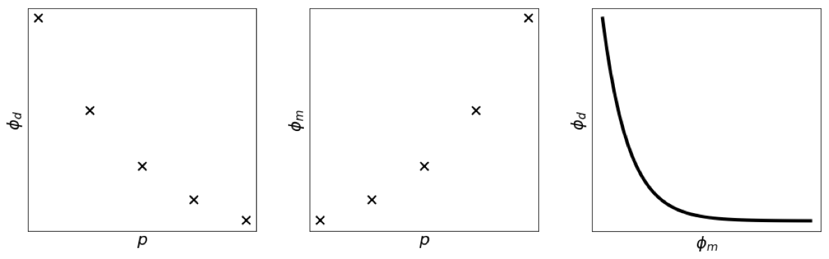
ϕ d = ∥ G m − d ∥ 2 \phi_d=\|\mathbf{Gm}-\mathbf{d}\|^2 ϕ d = ∥ Gm − d ∥ 2
ϕ m = ∥ m ∥ 2 \phi_m=\|\mathbf{m}\|^2 ϕ m = ∥ m ∥ 2
m c = ∑ i = 1 p ( u i T d λ i ) v i \mathbf{m}_c=\sum^p_{i=1}\left(\frac{\mathbf{u}_i^T\mathbf{d}}{\lambda_i}\right)\mathbf{v}_i m c = ∑ i = 1 p ( λ i u i T d ) v i
3.2 Ill-conditionedness ¶ m c = ∑ i = 1 p ( u i T d λ i ) v i \mathbf{m}_c=\sum^p_{i=1}\left(\frac{\mathbf{u}_i^T\mathbf{d}}{\lambda_i}\right)\mathbf{v}_i m c = ∑ i = 1 p ( λ i u i T d ) v i
Small singular value ↔ \leftrightarrow ↔
3.3 Truncated SVD ¶ If data are inaccurate the noise is also amplified by 1 λ i \frac{1}{\lambda_i} λ i 1
m c = ∑ i = 1 q ( u i T d λ i ) v i + ∑ i = q + 1 N ( u i T d λ i ) v i \mathbf{m}_c=\sum^q_{i=1}\left(\frac{\mathbf{u}_i^T\mathbf{d}}{\lambda_i}\right)\mathbf{v}_i + \sum^N_{i=q+1}\left(\frac{\mathbf{u}_i^T\mathbf{d}}{\lambda_i}\right)\mathbf{v}_i m c = ∑ i = 1 q ( λ i u i T d ) v i + ∑ i = q + 1 N ( λ i u i T d ) v i
So we simply use m c = ∑ i = 1 q ( u i T d λ i ) v i \mathbf{m}_c=\sum^q_{i=1}\left(\frac{\mathbf{u}_i^T\mathbf{d}}{\lambda_i}\right)\mathbf{v}_i m c = ∑ i = 1 q ( λ i u i T d ) v i
Truncated SVD treats/takes care of issues caused by non-uniqueness and ill-conditioning
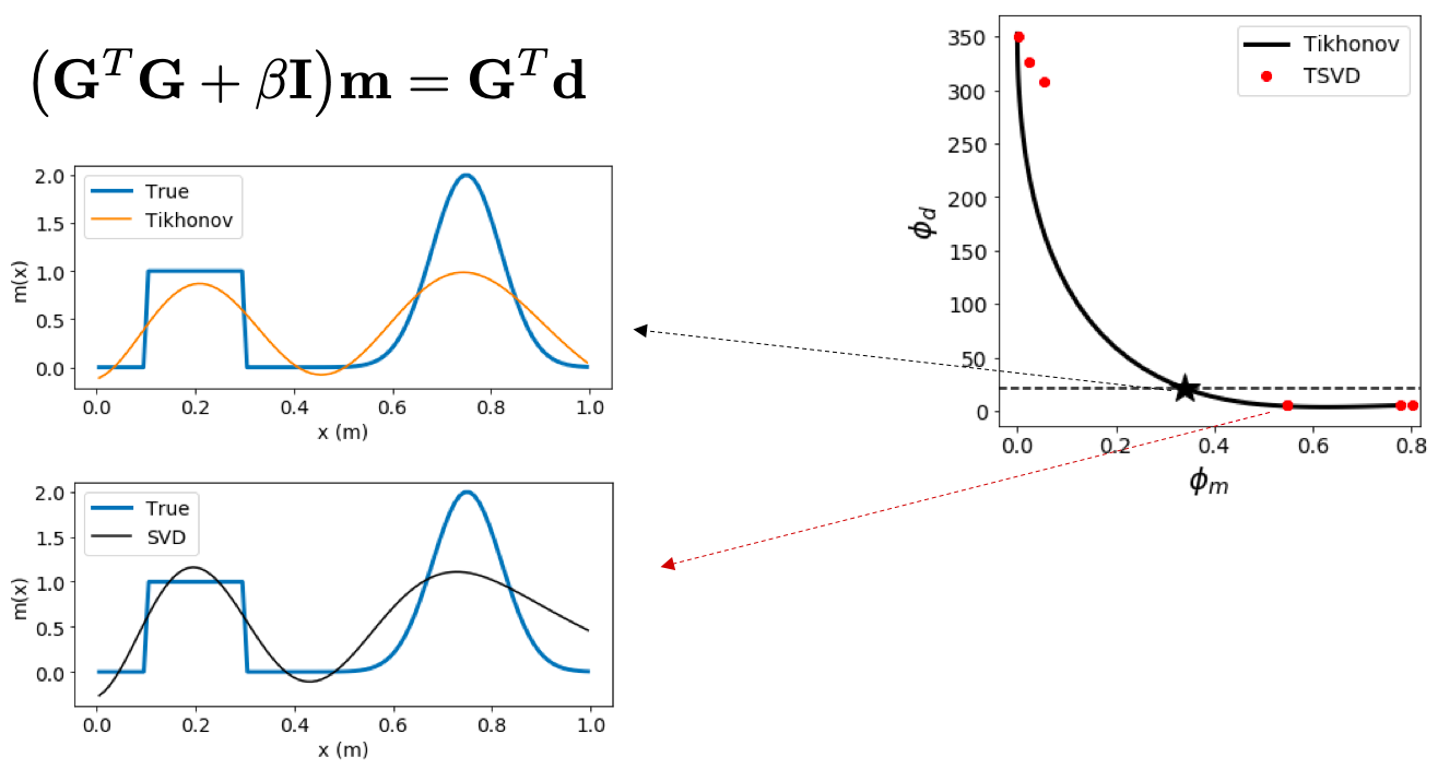
3.4 Consider Tikhonov Solution ¶ Data misfit ϕ d = ∥ G m − d ∥ 2 \phi_d=\|\mathbf{Gm}-\mathbf{d}\|^2 ϕ d = ∥ Gm − d ∥ 2
Regularization (Model norm?) ϕ m = ∥ m ∥ 2 \phi_m=\|\mathbf{m}\|^2 ϕ m = ∥ m ∥ 2
Minimize ϕ = ϕ d + β ϕ m = ∥ G m − d ∥ 2 + β ∥ m c ∥ 2 \begin{aligned}\phi&=\phi_d+\beta\phi_m\\ &=\|\mathbf{Gm}-\mathbf{d}\|^2+\beta\|\mathbf{m}_c\|^2\end{aligned} ϕ = ϕ d + β ϕ m = ∥ Gm − d ∥ 2 + β ∥ m c ∥ 2
Minimum ∇ g = ∇ m ϕ = 0 \nabla\mathbf{g}=\nabla_m\phi=0 ∇ g = ∇ m ϕ = 0
Differentiate with respect to vector ∂ ϕ ∂ m = 2 G T ( G m − d ) + 2 β m = 0 \frac{\partial\phi}{\partial\mathbf{m}}=2\mathbf{G}^T(\mathbf{Gm}-\mathbf{d})+2\beta\mathbf{m}=0 ∂ m ∂ ϕ = 2 G T ( Gm − d ) + 2 β m = 0
So ( G T G + β I ) m = G T d (\mathbf{G}^T\mathbf{G}+\beta\mathbf{I})\mathbf{m}=\mathbf{G}^T\mathbf{d} ( G T G + β I ) m = G T d G T G \mathbf{G}^T\mathbf{G} G T G ( M × M ) (M\times M) ( M × M ) r a n k ( G ) ≤ N , M > N rank(\mathbf{G})\leq N, ~M>N r ank ( G ) ≤ N , M > N β > 0 \beta>0 β > 0 β I \beta\mathbf{I} β I ≥ β \geq\beta ≥ β
Solve A m = b \mathbf{Am}=\mathbf{b} Am = b A = G T G + β I \mathbf{A}=\mathbf{G}^T\mathbf{G}+\beta\mathbf{I} A = G T G + β I b = G T d \mathbf{b}=\mathbf{G}^T\mathbf{d} b = G T d
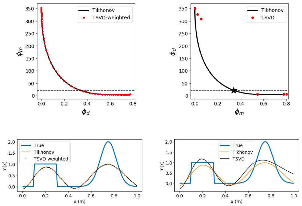
3.4.0.1 Tikhonov solution v TSVD ¶ 3.4.1 Tikhonov, TSVD, weighted TSVD ¶ ( G T G + β I ) m = G T d (\mathbf{G}^T\mathbf{G}+\beta\mathbf{I})\mathbf{m}=\mathbf{G}^T\mathbf{d} ( G T G + β I ) m = G T d
Exact correspondence is obtained by modifying to include weights
m c = V T Λ − 1 U d \mathbf{m}_c=\mathbf{VT\Lambda}^{-1}\mathbf{Ud} m c = VTΛ − 1 Ud
m c = ∑ i = 1 p t i ( u i T d λ i ) v i \mathbf{m}_c=\sum^p_{i=1}t_i\left(\frac{\mathbf{u}_i^T\mathbf{d}}{\lambda_i}\right)\mathbf{v}_i m c = ∑ i = 1 p t i ( λ i u i T d ) v i
T = ( t 1 ⋱ t p ) , 0 ≤ t i ≤ 1 \mathbf{T} =\begin{pmatrix} t_1& & \\ & \ddots & \\ & & t_p \end{pmatrix},~~0\leq t_i\leq 1 T = ⎝ ⎛ t 1 ⋱ t p ⎠ ⎞ , 0 ≤ t i ≤ 1
t i = λ i 2 λ i 2 + β t_i=\frac{\lambda_i^2}{\lambda_i^2+\beta} t i = λ i 2 + β λ i 2
4 Summary ¶ G m = d \mathbf{Gm}=\mathbf{d} Gm = d
G = U Λ V T \mathbf{G}=\mathbf{U\Lambda V}^T G = UΛV T
m c = ∑ i = 1 p t i ( u i T d λ i ) v i \mathbf{m}_c=\sum^p_{i=1}t_i\left(\frac{\mathbf{u}_i^T\mathbf{d}}{\lambda_i}\right)\mathbf{v}_i m c = ∑ i = 1 p t i ( λ i u i T d ) v i
Small singular values are associated with high frequency vectors in the model space and amplify the noise
Instabilities are handled by truncating, adjusting their influence (t i = λ i 2 λ i 2 + β t_i=\frac{\lambda_i^2}{\lambda_i^2+\beta} t i = λ i 2 + β λ i 2
Minimize ϕ = ϕ d + β ϕ m = ∥ G m − d ∥ 2 + β ∥ m c ∥ 2 \begin{aligned}\phi&=\phi_d+\beta\phi_m\\ &=\|\mathbf{Gm}-\mathbf{d}\|^2+\beta\|\mathbf{m}_c\|^2\end{aligned} ϕ = ϕ d + β ϕ m = ∥ Gm − d ∥ 2 + β ∥ m c ∥ 2
4.0.0.1 What does the solution tell us? ¶ A full data set can recover information about m ∥ \mathbf{m}^{\parallel} m ∥
The regularized solution is in a reduced region of the model space
The geophysical model lies outside of this region. To explore that we need to incorporate more information.