Defining the Inverse Problem

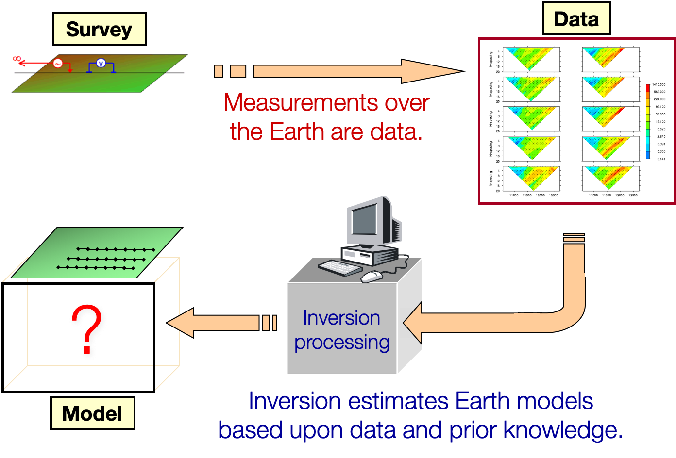
In a typical physical problem we perform an experiment to collect data and use those data to infer something about the earth. The procedure is schematically represented in the diagram below. The “inversion processing” is the computational component that links the observations to the unknown earth model.

Let $m$ be a generic symbol for the physical property or parameters that are being sought. We refer to $m$ as the “model”. A more rigorous statement of the inverse problem is: “Given observed data, $d_{j}^{obs}$, where $j=1,\dots,N$, an estimate of their uncertainties, $\epsilon_j$, and the ability to carry out forward modelling,

find the model that generated the data”. The quantity $\mathcal{F_j}$ is the forward modelling operator that was explained in Inverse Theory Overview. It encompasses the physical equations, geometries and all details about the source and receiver.

Solving an inverse problem using optimization theory is a multi-step process and in this section we look at each component in detail. It suffices to work with a simple synthetic example to establish fundamental principles that will be essential for every inverse problem we encounter. We first develop the forward modelling.